

Introduction
A store plans a 15% price cut on one product for the next four weeks, and the category manager needs order quantities for three related products: the promoted product itself, an alternative product customers might have bought instead, and a related product often bought alongside it. A promotion rarely affects just one product. Lowering one price can:- Increase sales of the promoted product
- Reduce sales of an alternative product through cannibalization — shoppers switch to the cheaper option instead of buying both
- Increase sales of a related product through cross-selling — shoppers who come for the promotion pick up companion items too
- How could a promotion change demand across a product group?
- How often could several products need replenishment at the same time?
With coupled simulation, one
sample_id represents one possible future for the
whole product group. The promoted, alternative, and related products all belong
to the same scenario.What You’ll Learn
- How to simulate a group of related products together with
multivariate=True - How to measure promotion lift, cannibalization, and cross-selling from simulated paths
- Why simulating products separately understates shared-demand risk
- How to turn a set of simulated futures into ordering decisions
How to Plan a Promotion with Coupled Simulation

Step 1: Import Packages
Import the required packages and initialize a Nixtla client:Step 2: Load the Product-Group Data
The example uses three years of daily sales for the three products. Every row carries all three prices, so when the promoted product’s price changes, the demand simulation for every product can respond. The data is generated rather than observed — that way the product relationships are known exactly, and the simulation’s answers can be checked against them (see the technical notes for how, and why, the data was built).Create the example data
Create the example data
The history covers 3,285 rows across the three products, from January 1, 2023
through December 30, 2025.
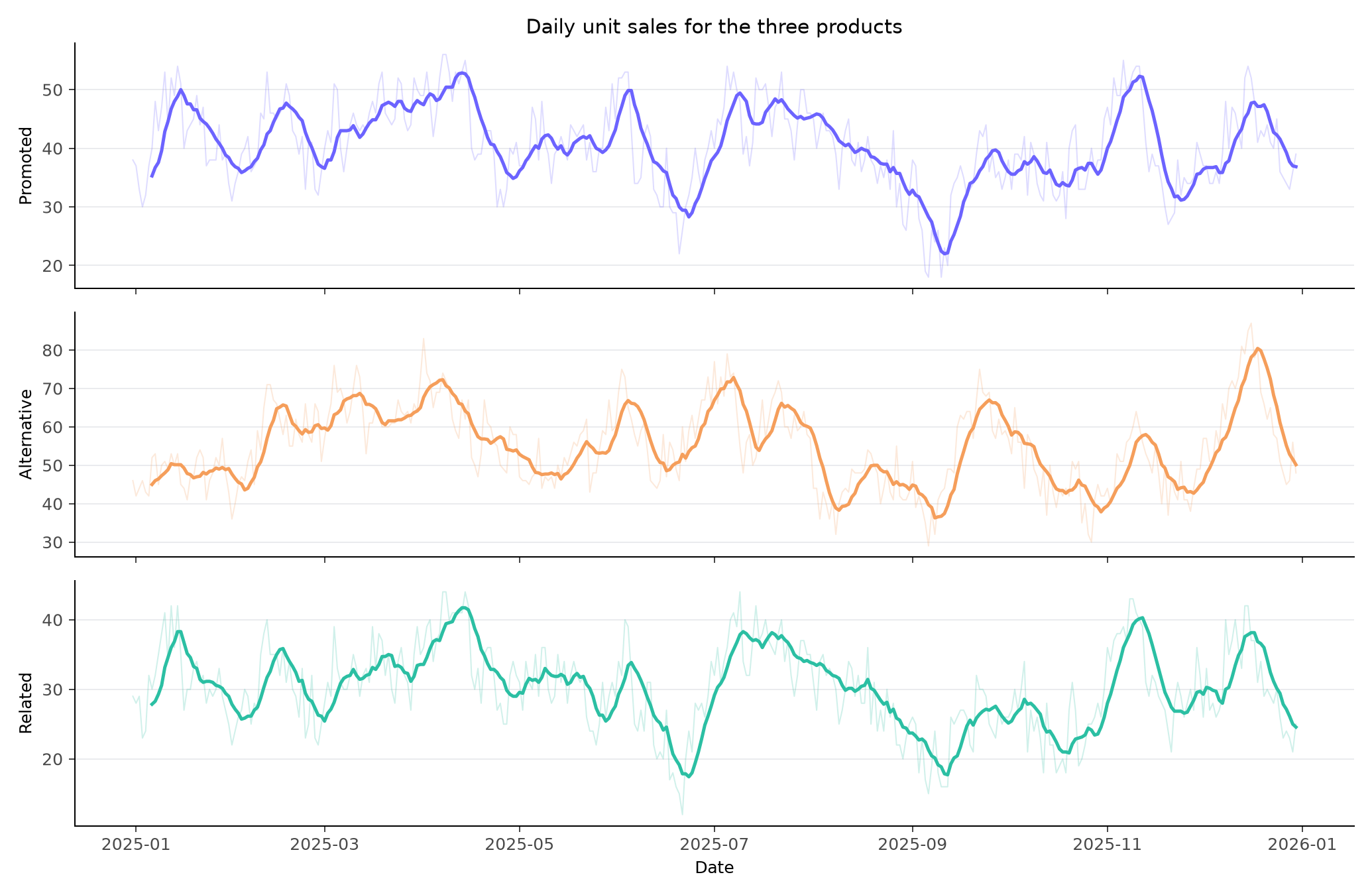
Light lines show daily sales; bold lines show seven-day averages over the final year of history.
Step 3: Define the Promotion
The next 28 days carry regular prices. Create a second plan with the promoted product’s price reduced by 15%, leaving the other prices unchanged:Step 4: Simulate the Product Group Under Both Plans
Generate 500 possible futures for all three products, first at current prices, then with the promotion:sample_id=12 contains one 28-day future for each of the three products.
multivariate=True changes two things at once. TimeGPT 2.1 forecasts the
products jointly, so each product’s forecast distribution can reflect the
others, and the sample paths are coupled, so one sample_id is one future for
the whole group. Both differences matter below.Step 5: Measure Lift, Cannibalization, and Cross-Selling
Product demand cannot be negative, so clip values at zero before calculating unit totals:
The promoted product gains approximately 66 units. The related product gains
approximately 42 units — the cross-selling signal. The alternative product
loses approximately 179 units — the cannibalization signal. All three
directions match the relationships built into the data (the
technical notes compare the sizes too).
This changes the business interpretation. Looking only at the promoted product
suggests a successful promotion. Looking at the complete product group shows that
the alternative product loses more units than the other two gain combined.
Step 6: Estimate Shared-Demand Risk
To see what simulating the products together changes, generate the promotion paths once more with the products simulated separately: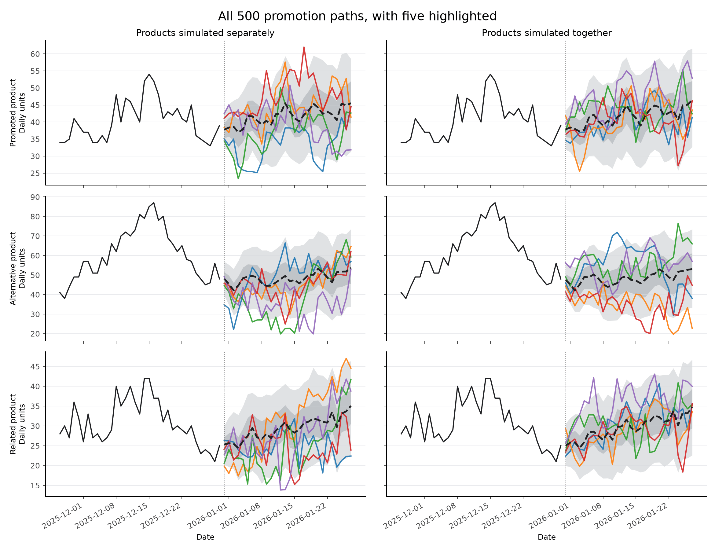
Shaded bands cover the 25th–75th and 5th–95th percentiles of all 500 paths, and dashed lines show the median. Five individual paths are drawn on top so that one product-group scenario can be followed. Each row shares a y-axis so the two columns are directly comparable.
The two runs use different seeds on purpose. Reusing one seed can return
identical paths for the first product in both runs, which would make one row of
the chart above appear twice. The technical notes explain
why.
What is the chance that at least two products experience high demand on the same day during the promotion?For this example, “high demand” means demand above that product’s 90th percentile in the separately simulated paths. The same thresholds are applied to both sets of paths.
Calculate the probability
Calculate the probability
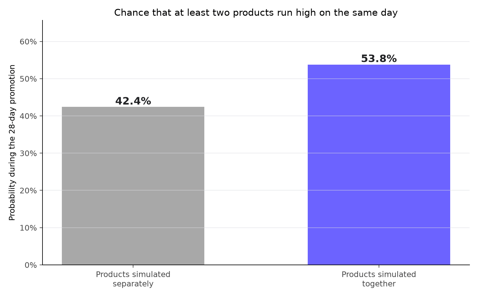
The calculation counts complete 28-day product-group paths.
Turn the Result into a Retail Decision
This example suggests three actions:- Increase inventory for the promoted product.
- Prepare for additional related-product demand.
- Reduce the alternative product’s order or reconsider the discount if total product-group volume is the goal.
sample_id, producing a
distribution of profit instead of only a distribution of units.
With real sales data, a demand response like this is an association rather than
proof of a mechanism. Prices are usually set alongside promotions and seasonal
events, so a measured cross-product effect can reflect a shared calendar instead
of shoppers substituting. Use experiments or basket data when you need to
establish why customers changed their purchases.
When Coupled Simulation Is Useful
Use coupled simulation when a decision combines several related series, such as:- Ordering a family of substitute or complementary products
- Staffing a shared fulfillment operation
- Estimating total category revenue
- Planning capacity for products promoted at the same time
Technical Notes
The planted relationships
Calling one product a substitute and another a complement is only honest if those relationships are actually in the data. Here they are written into the generator, so the labels are true by construction and the simulation’s answers can be checked against them.
Two more properties matter:
- Each product has its own price schedule, and the three do not move together. A promotion on one product is therefore a change the model can attribute to that product.
- An unobserved store-footfall factor lifts all three products on the same day. It is never passed to the model, so it survives as demand that moves together across the products — which is exactly what coupling has to reproduce. The products’ demand rank correlations over the history are 0.49 between the promoted and alternative products, 0.88 between the promoted and related products, and 0.47 between the alternative and related products.
Recovered versus planted effects
Compare the simulated changes from Step 5 with the planted effects. The cannibalization comes back almost exactly (−11.7% against a planted −11.5%), while the two gains come back at roughly half their planted size (+6.0% against +11.9%, and +5.4% against +15.0%). Forecasting a price level the model has not seen is conservative by nature, so treat these as directionally right and, for the gains, understated — not as exact elasticities.Why the seed differs between the coupled and separate runs
Both the coupled and the per-series shuffle draw their template windows from the same random state, so with a fixed seed the first product by name is reordered identically whethermultivariate is True or False — for this data it comes
back with exactly the same 500 paths. Varying the seed removes this overlap
when the two runs are compared visually.